Achieving Scalable Multilingual Semantic Search
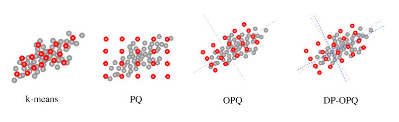
TABLE OF CONTENTS
- 1.Introduction#introduction
- 2.The Big Picture#the-big-picture
- 2.1.Seq2Seq#seq2seq
- 2.2.The BERT Family#the-bert-family
- 2.3.Approximate Nearest Neighbors#approximate-nearest-neighbors
- 3.Examples#examples
- 3.1.Computing Sentence Embeddings#computing-sentence-embeddings
- 3.2.Semantic Search#semantic-search
- 3.3.Using FAISS#using-faiss
- 3.4.Simple System#simple-system
- 4.Final Words#final-words
- 5.Resources#resources
Introduction
This article is based on the work I did for a project that involved millions of documents in different languages. The goal was to build a system that could retrieve documents in multiple languages based on an input query in one language. The purpose of this article is to give a very high-level picture of concepts, ideas, and tools that could be used for building such a system.
Most of the things mentioned here are connected to Natural Processing Language (NLP) field. However, as you will see, this type of a system could be used for multiple problems, not just for NLP, as it relies on vector representation and efficient vector similarity matching.
If you are completely new to the NLP field some of the things mentioned here will be unclear. I'll do my best to give small explanations and reference material where you can find more information.
It's not possible to cover everything since this topic is elaborate and a subject to constant change but I'll try to go over the following topics:
- Big Picture - a brief overview of some NLP/ANN concepts
- Techniques - techniques and methods for dealing with large amount of high-dimensional vector representations
- Examples - open source libraries and code snippets
The Big Picture
Seq2Seq
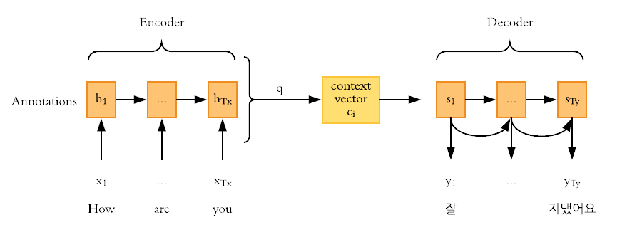
We can look at the translation as a sequence-to-sequence (seq2seq) problem which translates a sequence from one domain to a sequence in another domain. This is achieved using encoder-decoder infrastructure, where a sentence is an input for encoder which encodes it to a fixed-length internal representation that is used by decoder to give an output.
Neural networks, especially RNNs are well suited for this task. However, there's a problem. As sentences become larger, we notice a decline in the performance of the network, also known as vanishing gradient problem. This gave birth to the new mechanism called attention which tries to solve this by focusing on parts of input sequences. There are several attention mechanisms and you can take a deep dive into them by reading: Attention in NLP.
Self-attention is one of the attention mechanisms that was used to create a novel encode-decoder architecture: the transformer. It's detailed in the Attention Is All You Need paper and it completely changed the NLP field. It introduced a new approach to solving seq2seq tasks while handling long-range dependencies with ease. This architecture relies solely on the self-attention mechanism without using sequence-aligned RNNs or convolution. The transformer is highly parallelizable and requires less time to train.
If you would like to learn more about self-attention please see: Illustrated: Self-Attention.
The BERT Family
The BERT stands for Bidirectional Encoder Representations from Transformers, and is a language representation model based on Transformer encoder network. As mentioned above, that network can process long texts efficiently because it relies on the self-attention mechanism.
The network contains 12 successive transformer layers, 12 attention heads (each layer has one), 768 hidden units, and 110 million parameters.
Of course, the actual numbers depend on the type of the model: base, large, etc. If you'd like to find out more, I suggest reading English Bert.
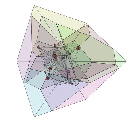
Here's a nice 3D image that depicts the network:
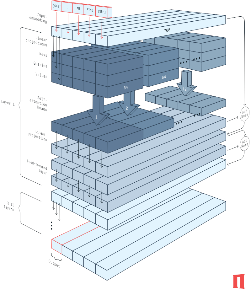
The output of this model is a high-dimensional vector. The number of dimensions is equal to hidden units i.e. 768.
This model has been released to the public with pre-trained weights. Pre-training a model is quite expensive, takes a lot of time, and requires a huge amount of data. That's why the pre-trained weights are important and we can easily fine tune the model for our purposes and specific aims.
There are other models based on BERT such as: DistilBERT, BioBERT, CamemBERT, VideoBERT, VilBERT, ALBERT, RoBERTa, DocBERT and many more.
If you'd like to read more about the different BERT models, I would suggest Domain-Specific BERT Models.
Out of this plethora of models I would distinguish XLMRoBERTa. XLM stands for Cross-lingual Language Model and RoBERTa for Robustly Optimized BERT Pretraining Approach.
XLMRoBERTa is a multilingual model and is trained on 100 different languages.
What makes it so awesome is that it doesn't require lang tensor to understand
which language is used since it's able to determine the correct language based
on input ids.
Approximate Nearest Neighbors
Basics
As amount of data grows each day and data applications struggle to be responsive and efficient, some business requirements and data operations as similarity search create insurmountable issues.
There are different methods of searching, but as we scale to millions or billions data entries we have to implement optimized solutions such as approximate nearest neighbors (ANN) algorithms. The trick here is that we are forced to trade some accuracy in order to achieve a similarity search that can be orders of magnitude faster.
ANN techniques speed up the search by preprocessing the data into an efficient index. This is achieved by transforming vectors before they are indexed, such as dimensionality reduction, vector rotation, and encoding to a much compact form in order to construct the actual index etc.
There are several popular methods of building ANNs, some of which are:
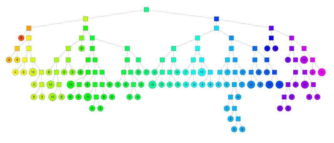
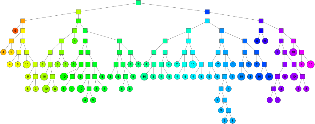
- Encoding using trees: It creates a binary tree that partitions a vector space. The trick here is that the points that are close to each other in the vector space are most likely to be close to each other in the tree. The popular implementation of this approach is Annoy, which is developed and used by Spotify to implement music recommendation system.
If you are interested in details of this approach, please see Nearest neighbors and vector models
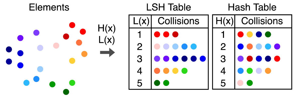
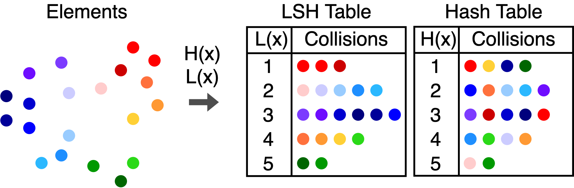
- Encoding using LSH: Locality-sensitive hashing is used to create "buckets" of similar input items which enables this technique to be used for data clustering and implementation of approximate nearest neighbors. The popular implementation of this approach is FAISS. When applied to vector space LSH will result in partition of vector space into buckets based on similarity between vectors.
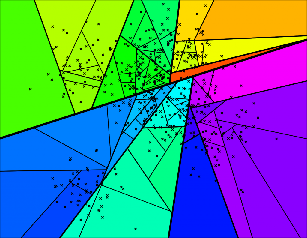
- Encoding using Quantization: Another approach is to map the vector space into a smaller collection of representative vectors (also called codebook). For example we could find these vector by running a K-means clustering algorithm. This results in a partitioning of the vector space into Voronoi cells where the representative vector is a cluster centroid of a cell.
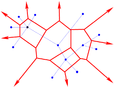
This allows us to query only the representative vectors. Of course, this approach lowers the accuracy of the search but it significantly increases the response time.
All these methods approximate nearest neighbors and speed up similarity search but when we deal with millions or billions of documents, these representative vectors can be quite heavy, especially if they are high dimensional (which happens in NLP).
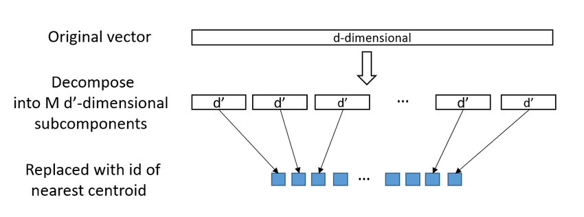
Another method to lower the space required for these vectors is Product Quantization which basically approximates the distance/similarity calculation by compressing the vectors. This is achieved by splitting the vector into equal length subvectors and then assigning these subvectors to its nearest centroids.
FAISS
FAISS stands for Facebook AI Similarity Search and is a C++ library (with Python bindings) that implements efficient similarity search when the number of vectors goes up to millions or billions. It also comes with built-in GPU optimization for any CUDA-enabled machine.
Let's say we have a set of vectors
where
When we look at types of indexes
we can see that we have over 10 types to choose from: IndexFlatL2,
IndexFlatIP, IndexHNSWFlat, IndexIVFFlat, IndexLSH, IndexPQ,
IndexIVFScalarQuantizer, IndexIVFPQ, etc.
So, how do we know which one to use?
It really depends on the use case. It's obvious that we will always have to trade some accuracy for speed but also the number of vectors plays a huge role in choosing the right index type. To better understand the meaning of index names, let's cover the important ones:
- Flat is used to label indexes that store whole vectors without compression
For example IndexFlatL2 measures
- IVF stands for inverted file index and is used to partition vector space
into
partitions
However, here we have to train the index. This is required in order to add groupings and build the index. Partitioning of vector space speeds up the process of querying since we are first matching the main vector of each cluster, or if you like to think in visual terms, each Voronoi cell.
Unfortunately, this approximation can lead to suboptimal results. One way to
improve it is to increase nprobe parameter, which defines the number of
nearby cells to search. Think of it as probing cells, if nprobe is 5, we
visit 5 cells and get the one which has the best result, if we probe 15 cells,
the probability of getting the best cells with best vectors in it increases.
-
LSH stands for Locality Sensitive Hashing which we already mentioned. Index can also be built using LSH to partition vector space and use cell-probe methods to probe partitions
-
PQ stands for Product Quantization as mentioned earlier and is used to compress vectors. This is used if storing the whole vector is too expensive and is considered to be most useful indexing structure for large-scale search
There are more details about choosing the best index structure for your use case Guidelines to choose an index.
Usually the index is stored in RAM, but if it gets too large it can be store on a disk, which of course has some performance impact.
What makes FAISS' API really awesome for developing applications is that it
can return not just the nearest neighbor but also
For more details about FAISS, check out these two excellent articles:
Examples
Let's play around with these concepts using an open source library: sentence-transformers, that provides an easy method to compute dense vector representations for sentences, paragraphs, and images. This framework can be used for: Computing Sentence Embeddings, Semantic Textual Similarity, Clustering and many more.
To install sentence-transformers you'll need python >= 3.6,
PyTorch >= 1.6.0, and transformers >= v4.6.0.
Computing Sentence Embeddings
To use pretrained models, specify the model_name parameter for
SentenceTransformer.
The models are hosted on HuggingFace Model Hub, the code will automatically
pull the model and cache it locally:
from sentence_transformers import SentenceTransformer
model = SentenceTransformer('model_name')
The SentenceTransformer has encode method that computes the embeddings, we
can pass a str or List[str]:
sentences = [
    "If numbers aren't beautiful, I don't know what is.",
    "Another roof, another proof.",
    "We'll continue tomorrow - if I live.",
]
embeddings = model.encode(sentences)
print(type(embeddings))                 # <class 'numpy.ndarray'>
print(embeddings.shape)                 # (3, 768)
We can see that we get 3 vectors with 768 dimensions, as we expected.
Semantic Search
Now that we know how to get the embeddings, let's choose a general purpose
model, for example all-distilroberta-v1, calculate embeddings and use
them to find top 3 similar sentences using a set of sentences and a query:
To get more information on pretrained model, please see Pretrained Models.
from sentence_transformers import SentenceTransformer, util
import torch

model = SentenceTransformer('all-distilroberta-v1')

sentences = [
    "Writing a list of random sentences is harder than I initially thought it would be.",
    "Nobody has encountered an explosive daisy and lived to tell the tale.",
    "She hadn't had her cup of coffee, and that made things all the worse.",
    "That is an appealing treasure map that I can't read.",
    "She saw the brake lights, but not in time.",
    "The chic gangster liked to start the day with a pink scarf.",
    "She wondered what his eyes were saying beneath his mirrored sunglasses."
]
query = "My mornings begin with a coffee"

embeddings = model.encode(sentences, convert_to_tensor=True)
query_embedding = model.encode(query, convert_to_tensor=True)

cos_scores = util.cos_sim(query_embedding, embeddings)[0]
top_results = torch.topk(cos_scores, k=3)

for score, idx in zip(top_results[0], top_results[1]):
    print(sentences[idx], "(Score: {:.4f})".format(score))
The result is:
She hadn't had her cup of coffee, and that made things all the worse. (Score: 0.3603)
The chic gangster liked to start the day with a pink scarf. (Score: 0.2459)
Writing a list of random sentences is harder than I initially thought it would be. (Score: 0.1719)
Using FAISS
The util.cos_sim(a[i], b[j]) computes the cosine similarity for all i and
j and we already know that this won't work if we have large amount of
documents.
For presentational purposes, let's play with a collection of email messages of employees in the Enron Corporation which can be found at AESLC. We won't deal with cleaning and preparing the data, that would make article too long, and accuracy is not the main focus of this article.
Since these emails can be very long and we are using BERT-based model which has sentence length of 512 word pieces, we have to implement a simple solution that will divide a sentence into chunks and compute embeddings for each chunk then combine it. I suggest you take a look at: How to use Bert for long text classification? and Long-texts-Sentiment-Analysis-RoBERTa.
To get these chunks we can use:
def _get_chunks(text, length=200, overlap=50):
    l_total = []
    l_partial = []
    text_split = text.split()
    n_words = len(text_split)
    splits = n_words // (length - overlap) + 1
    if n_words % (length - overlap) == 0:
        splits = splits - 1
    if splits == 0:
        splits = 1
    for split in range(splits):
        if split == 0:
            l_partial = text_split[:length]
        else:
            l_partial = text_split[
                split * (length - overlap) : split * (length - overlap) + length
            ]
        l_final = " ".join(l_partial)
        if split == splits - 1:
            if len(l_partial) < 0.75 * length and splits != 1:
                continue
        l_total.append(l_final)
    return l_total
These chunks have to be processed and combined, there are multiple ways to do this, for example joining them into one LSTM layer, but for the sake of simplicity let's just calculate the mean.
def calculate_embeddings(text):

    chunks = _get_chunks(text)
    embeddings = np.empty(
        shape=[len(chunks), 768],
        dtype="float32",
    )
    for index, chunk in enumerate(chunks):
        chunk_embedding = model.encode(
            chunk,
            convert_to_numpy=True,
        )
        embeddings[index:] = chunk_embedding
    mean = embeddings.mean(axis=0)
    mean_normalized = mean / np.linalg.norm(mean)

    return mean_normalized
In the AESLC train dataset there are 14436 emails. To quickly test the idea,
let's use only the emails that start with s, calculate embeddings, generate
an uuid for email that could be used to identify an email, and then save that
information in a pickle file:
model = SentenceTransformer('all-distilroberta-v1')
emails_path = "AESLC/enron_subject_line/train"
emails = []

for file in os.listdir(emails_path):
    if file.startswith("s"):
        with open(os.path.join(emails_path, file)) as f_in:
            email_text = f_in.read()
            emails.append(email_text)

email_embeddings = [calculate_embeddings(x) for x in tqdm(emails)]
email_uuids = [str(uuid.uuid4()) for _ in emails]

with open("emails.pkl", "wb") as f_out:
    pickle.dump(
        {
            "email_uuids": email_uuids,
            "email_texts": emails,
            "email_embeddings": email_embeddings
        },
        f_out
    )
Now that we have embeddings we can load them, define, train, and search a FAISS index:
import faiss
import pickle
import numpy as np
from sentence_transformers import SentenceTransformer

# Load stored embeddings
with open("emails.pkl", "rb") as f_in:
    data = pickle.load(f_in)
    email_texts = data["email_texts"]
    email_uuids = data["email_uuids"]
    email_embeddings = data["email_embeddings"]

# Define Index properties
top_k_hits = 3
embedding_size = 768
n_clusters = 10
quantizer = faiss.IndexFlatIP(embedding_size)
index = faiss.IndexIVFFlat(quantizer, embedding_size, n_clusters, faiss.METRIC_INNER_PRODUCT)
index.nprobe = 3

# Train index and add embeddings
embeddings = email_embeddings / np.linalg.norm(email_embeddings, axis=1)[:, None]
index.train(embeddings)
index.add(embeddings)

# Process Query
model = SentenceTransformer('all-distilroberta-v1')
query = ""      # <- define a query
query_embeddings = model.encode(query)
query_embeddings = query_embeddings / np.linalg.norm(query_embeddings)
query_embeddings = np.expand_dims(query_embeddings, axis=0)

# Search Index
distances, embedding_ids = index.search(query_embeddings, top_k_hits)
hits = [{'id': _id, 'score': score} for _id, score in zip(embedding_ids[0], distances[0])]
hits = sorted(hits, key=lambda x: x['score'], reverse=True)

for hit in hits[0:top_k_hits]:
    print("====================")
    print("- Score: ", hit['score'])
    print("- Email UUID: ", email_uuids[hit['id']])
    print("- Email Text:")
    print("---------")
    print(email_texts[hit["id"]])
    print("---------")
To test it, let's try to query it with a part of some other email which is not in the index:
Please see the attached spreadsheet for a  trade by trade list and a summary.
We have also included a summary of gas  daily prices to illustrate the value of San Juan based on several spread  relationships.
The two key points from this data are as follows:   1.
The high physical prices on the 26th & 27th (4.75,4,80) are much greater  than the high financial trades (4.6375,4.665) on those days.
2.
Results:
====================
- Score:  0.4753121
- Email UUID:  3ff56d47-fcb0-4ff5-aef0-cbb54d5a0dec
- Email Text:
---------
The Dow Jones report is compiled of data sent from many different  counterparties.
The lovely people at Dow Jones painstakingly analyze the data  to ensure its accuracy.
Averaged together, these prices become the Dow Jones  daily index price.
And that's the long and short of it.
The process, as you've guessed by now, is a little more complicated than  that.
For one thing, Dow Jones looks at each counterparty's sales to reach an  average of all the prices.
It would be redundant for each counterparty to  ALSO report their purchases from each other.
Therefore, when calculating the  Dow Jones data, we only include purchases from counterparties who ARE NOT  participants in the Dow Jones survey.
Following is a simple example:  Participant List  NP-15 Purchases  NP-15 Sales  Reported NP-15 Purchases  Reported NP-15 Sales Sempra  Sempra - $250   Sempra - $250  Avista - $270   Sempra - $250 Duke   Duke - $260   Duke - $260      Duke - $260 Enron   Avista - $270   Avista - $270      Avista - $270  Now that's simple!
Following is the participant list for Dow Jones' survey of trading at NP-15  and SP-15 delivery points.
Deals with these counterparty names need to be  excluded from the calculation of PURCHASES at NP-15 and SP-15 delivery points.
American Electric Power - Amerelecpo Avista Energy - Avistaene Duke Energy Trading and Marketing - Dukeenetra El Paso Merchant Energy Enron Power Marketing, Inc. - EPMI Idaho Power Company - Idacorpene PacifiCorp - PACE Pacific Gas & Electric Company - PG&E Powerex Corp. - PWX Puget Sound Energy, Inc. - PSPL Mirant Americas Energy Marketing (formerly Southern Company Energy Marketing)  - SCEM TransAlta Energy Marketing (US) Inc. - Transalt  So I've probably succeeded in confusing you even more, but please feel free  to come bug me with questions.
Good luck!
Kate

@subject
Dow Jones Report
---------
====================
- Score:  0.46080276
- Email UUID:  7f5f2455-510e-484b-8918-041b31c2db8b
- Email Text:
---------
The attached document contains the EPMI average prices for all delivery  points for Sun., March 25, and Mon., March 26.
Please let me know if you have  any problems opening the document or reading it.
The worksheet should look  identical to the fax I send each day.
An additional worksheet shows a detail  of each deal volume and price.
I'm in the habit of excluding the counterparty  names (to save time) because I'm the only one who looks at this sheet  normally; but if you'd like me to start e-mailing instead of faxing the  prices I will begin entering the counterparty names as well.
Thanks,

@subject
Dow Jones Index 3-26
---------
====================
- Score:  0.43980664
- Email UUID:  47cfb6a0-74dd-4dc1-9f42-2ca532f1132f
- Email Text:
---------
Holden & Lisa -  Per Holden, I've changed deal 630176 from a price of $170 to $197.
Terms and reasons are as follows:       6/4/01  STSW buys EPE   49 mw/HLH        The other side of this deal is a sale to El Paso for $204.
Kathy questioned the invoice she received from Houston this month, because the breakdown of transmission costs and fees we had given her (regarding buy-resales done by your desk on 6/1, 6/2, and 6/4) amounted to a spread of $14.06.
The deals we entered into our system, and subsequently billed El Paso for, amounted to spreads of $14.06 for 6/1,       $11.06 for 6/2, and $34 for 6/4.
To remedy this, and extend a gesture of apology for the mistake, we've changed our buy from El Paso on  the 4th to a price of $197, leaving a spread of $7 to cover our transmission costs.
I've explained this to Kathy at El Paso and Amy in Settlements, and wanted to give both of you a record of the change as well.
Please let      me know if you have any questions.
Thanks,

@subject
June EPE Buy-Resales
---------
Query with trade lists and spreadsheets, returns emails which topics revolve around prices, Dow Jones, sales, etc, which is not surprising.
Simple System
Let's say that you want to implement semantic search in your application that has the usual frontend and backend infrastructure. One of the ways to test ideas is to create a simple system that will use FAISS as an API.
The easiest way to achieve that is to wrap a FAISS index with something like Flask. The idea is to have a Flask server that is completely decoupled from your backend, it will search the FAISS index that you created and your backend can create API calls to the flask server.
This can be further integrated with a full-text search engine like Elasticsearch. Elasticsearch's support for text/sentence embeddings is fairly new, limited, and a field of ongoing work (Ref: Text similarity search with vector fields ). There are plugins that can implement ANN solutions in Elasticsearch as described here: Scalable Semantic Vector Search with Elasticsearch. However, as an exercise we can implement ANN separately and keep Elasticsearch's native search possibilities for certain types of queries.
It would look like this:
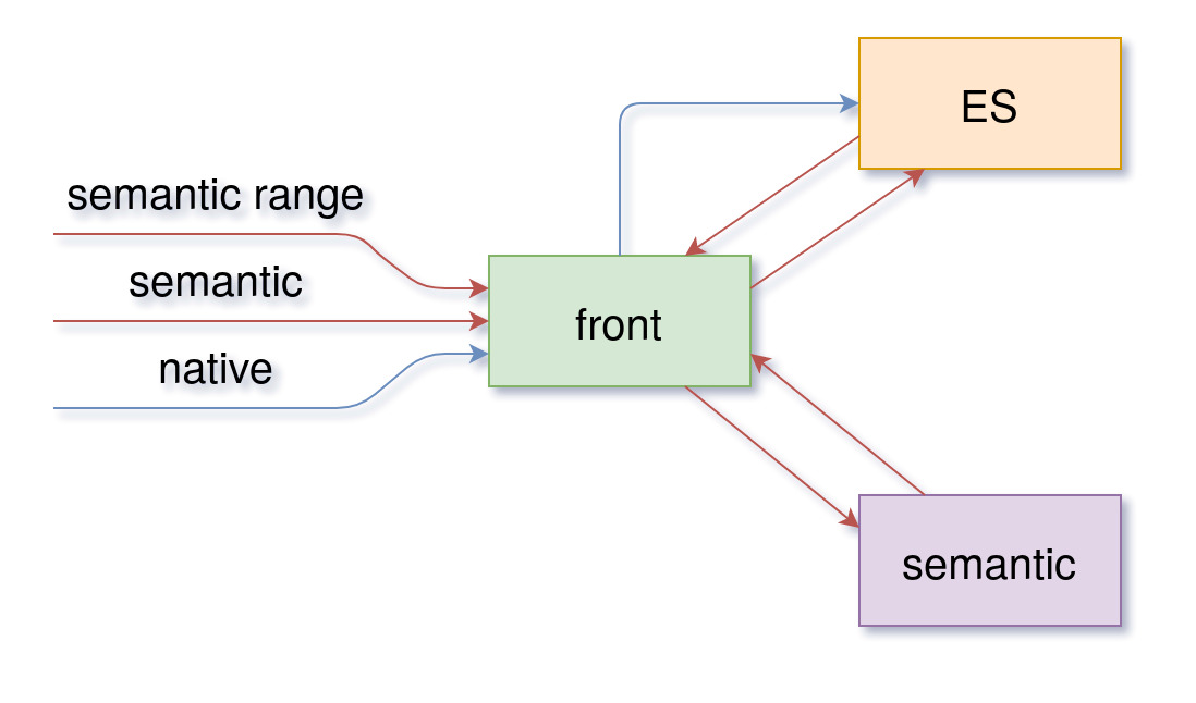
Illustration of a simple system idea
front represents an API that communicates with Elastisearch and a FAISS API - labeled as semantic, it proxies API calls based on queries that can be:
- native - full-text Elasticsearch queries
- semantic - semantic query that returns first top N hits
- semantic range - semantic query that returns all articles in a defined range of similarity score
When your application makes a semantic query, front will first create a call to semantic to get the document ids that are either first top N hits or in a defined range of similarity score, and then it will get those documents from Elasticsearch (or any other engine/database).
If you would like to learn more about this and checkout the code, please see the sample project on my github: Semantic Search System.
Final Words
My aim was to give a brief introduction to what happens behind a semantic search system and how it works. Concepts are introduced at a very high level which, I hope, helps you see the big picture more clearly.
There are many details which I didn't cover. Dealing with different models, accuracy, different methods of processing long texts and many more play a significant role in performance of the search.
Examples are there to show you how you can play with these concepts, explore them and create toy applications. If you are interested in finding out more, please go through provided material and resources.
If you have any questions or suggestions, please reach out, I'm always available.