Understanding Big Data File Formats
TABLE OF CONTENTS
Introduction
As we all know, juggling data from one system to another, transforming it through data pipelines, storing, and later performing analytics can easily become expensive and inefficient as the data grows. We often think about scalability and how to deal with the 4Vs1 of data, making sure that our system can handle dynamic flows and doesn't get overwhelmed with the amount of data.
There are many aspects of Big Data systems that come into considerations when we talk about scalability. Not surprisingly, one of them is how we define the storage strategy. A huge bottleneck for many applications is the time it takes to find relevant data, processes it, and write it back to another location. As the data grows, managing large datasets and evolving schemas becomes a huge issue.
Whether we are running Big Data analytics on on-prem clusters with dedicated or bare metal servers, or on cloud infrastructure, one thing is certain: the way we store our data and which file format we use will have an immense impact. How we store the data in our datalake or warehouse is critical.
Among many things, choosing an appropriate file format can:
- Increase read/write times
- Split files
- Support schema evolution
- Support compression
In this article we will cover some of the most common big data formats, their structure, when to use them, and what benefits they can have.
AVRO
As we all know, to transfer the data or store it, we need to serialize it first. Avro is one of the systems that implements data serialization. It's a row-based remote procedure call and data serialization framework. It was developed by Doug Cutting2 and managed within Apache's Hadoop project.
It uses JSON for defining data types and serializes data in a compact binary format. Additionally, Avro is a language-neutral data serialization system which means that theoretically any language could use Avro.
Structure
An Avro file consists of:
- File header and
- One or more file data blocks
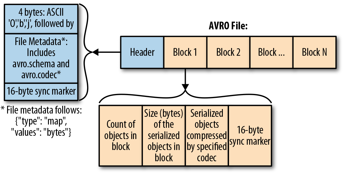
Header contains information about the schema and codec, while blocks are divided into:
- Counts of objects in a block
- Size of the serialized objects
- Objects themselves
If you are interested, take a look at Java implementation
Schema
Schema can be defined as:
- JSON string,
- JSON object, of the form:
{"type": "typeName" ...attributes...} - JSON array
or Avro IDL for human readable schema
typeName specifies a type name which can be a primitive or complex type.
Primitive types are: null, boolean, int, long, float, double,
bytes, and string.
There are 6 complex types: record, enum, array,
map, union, and fixed. Each of them supports attributes. In case of the
record type, they are:
name: name of the record (required)namespace: string that qualifies the namedoc: documentation of the schema (optional)aliases: alternative names of the schema (optional)fields: list of fields, where each field is a JSON object
The attributes of other complex types can be found in the
Apache Avro Specification
Now that we understand the structure of the schema, we can define it as, for example:
 {
   "namespace": "example.vladsiv",
   "type": "record",
   "name": "vladsiv",
   "doc": "Just a test schema",
   "fields": [
      {"name": "name", "type": "string"},
      {"name": "year",  "type": ["null", "int"]}
   ]
 }
Why Avro?
- It is a very fast serialization/deserialization format, great for storing raw data
- Schema is included in the file header, which allows downstream systems to easily retrieve the schema (no need for external metastores)
- Supports evolutionary schemas - any source schema change is easily handled
- It's more optimized for reading series of entire rows - since it's row-based
- Good option for landing zones where we store the data for further processing (which usually means that we read whole files)
- Great integration with Kafka
- Supports file splitting
Parquet
Apache Parquet is a free and open-source column-oriented data storage format and it began as a joint effort between Twitter and Cloudera. It's designed for efficient data storage and retrieval.
Running queries on the Parquet-based file-system is extremely efficient since the column-oriented data allows you to focus on the relevant data very quickly. This means that the amount of data scanned is way smaller which results in efficient I/O usage.
Structure
Parquet file consists of 3 parts:
- Header: which has 4-byte magic number
PAR1 - Data Body: contains blocks of data stored in row groups
- Footer: where all the metadata is stored
The 4-byte magic number PAR1, stored in the header and footer, indicates that
the file is in parquet format.
Metadata includes the version of the format, schema, information about the columns in the data which includes: type, path, encoding, number of values etc. The interesting fact is that the metadata is stored in the footer, which allows single pass writing.
So how do we read a parquet file? At the end of the file we have footer length, so the initial seek will be performed to read the length and then, since we know the length, jump to the beginning of the footer metadata.

Why is this important?
Since body consists of blocks and each block has a boundary, writing metadata at the end (when all the blocks have been written) allows us to store these boundaries. This gives us a huge performance when it comes to locating the blocks and processing them in parallel.
Each block is stored in the form of row groups. As we can see in the image above, row groups have multiple columns called: columnar chunks. These chunks are further divided into pages. The pages store values for a particular column and can be compressed as the values can repeat.
Schema
Parquet supports schema evolution. For example, we can start with a simple schema, and then add more columns as needed. By doing this, we end up with multiple Parquet files with different schemas. This is not an issue since the schemas are mutually compatible and Parquet supports automatic schema merging among those files.
When it comes to data types, Parquet defines a set of types that is intended to be as minimal as possible:
BOOLEAN: 1 bit booleanINT32: 32 bit signed intsINT64: 64 bit signed intsINT96: 96 bit signed intsFLOAT: IEEE 32-bit floating point valuesDOUBLE: IEEE 64-bit floating point valuesBYTE_ARRAY: arbitrarily long byte arrays.
These are further extended by Logical Types. This keeps the set of primitive types to a minimum and reuses parquet's efficient encodings. These extended types are:
- String Types:
STRING,ENUM,UUID - Numerical Types:
Signed Integers,Unsigned Integers,DECIMAL - Temporal Types:
DATE,TIME,TIMESTAMP,INTERVAL - Embedded Types:
JSON,BSON - Nested Types:
Lists,Maps - Unknown Types:
UNKNOWN- always null
If you are interested in details regarding Logical Types and encodings, please see: Parquet Logical Type Definitions and Parquet encoding definitions.
Why Parquet?
- When we are dealing with many columns but only want to query some of them - Since Parquet is column-based it's great for analytics. As the business expands we usually tend to increase the number of fields in our datasets but most of our queries just use a subset of them
- Great for very large amounts of data - Techniques like data skipping increase data throughput and performance on large datasets
- Low storage consumption by implementing efficient column-wise compression
- Free and open source - It's language agnostic and decouples storage from compute services (since most of data analytic services have support for Parquet out of the box)
- Works great with serverless cloud technologies like AWS Athena, Amazon Redshift Spectrum, Google BigQuery, Google Dataproc etc
ORC
Apache ORC (Optimized Row Columnar) is a free and open-source column-oriented data storage format. It was first announced in February 2013 by Hortonworks in collaboration with Facebook3.
ORC provides a highly efficient way to store data using block-mode compression based on data types. It has great reading, writing, and processing performance thanks to data skipping and indexing.
Structure
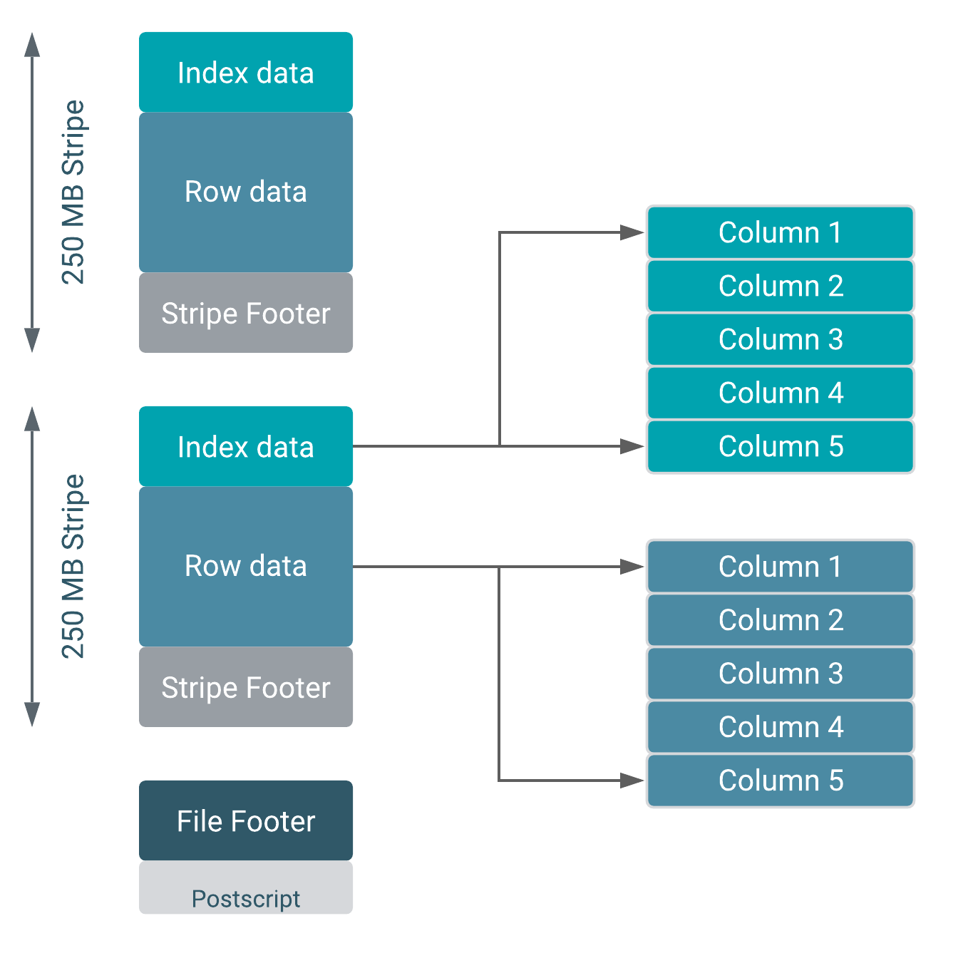
ORC file format consists of:
- Groups of row data called stripes
- File footer
- Postscript
The process of reading an ORC file starts at the end of the file. The final byte of the file contains the length of the Postscript. The Postscript is never compressed and provides the information about the file: metadata, version, compression etc. Once we parse the Postscript we can get the compressed form of the File Footer, decompress it, and learn more about the stripes stored in the file.
The File Footer contains information about the stripes, the number of rows per stripe, the type schema information, and some column-level statistics: count, min, max, and sum.
Stripes contain only entire rows and are divided into three sections:
- Index data: a set of indexes for the rows within the stripe
- Row data
- Stripe footer: directory of stream locations
What's important here is that both the indexes and the row data sections are in column-oriented format. This allows us to read the data only for the required columns.
Index data provides information about the columns stored in row data. It includes min and max values for each column, but also row positions which provide offsets that enable row-skipping within a stripe for fast reads.
For in-depth information about the ORC file format, see ORC Specification v1
Schema
Like Avro and Parquet, ORC also supports schema evolution. This allow us to merge schema of multiple ORC files with different but mutually compatible schemas.
ORC provides a rich set of scalar and compound types:
- Integer:
boolean,tinyint,smallint,int,bigint - Floating point:
float,double - String types:
string,char,varchar - Binary blobs:
binary - Date/time:
timestamp,timestampwith local time zone,date - Compound types:
struct,list,map,union
All scalar and compound types in ORC can take null values.
There is a nice example in the ORC documentation: Types, that illustrates how it works.
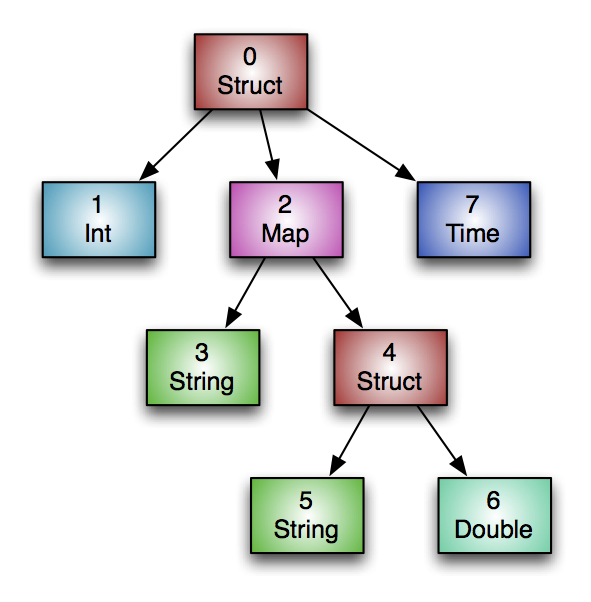
Let's say that we have the table Foobar:
create table Foobar (
 myInt int,
 myMap map<string,
 struct<myString : string,
 myDouble: double>>,
 myTime timestamp
);
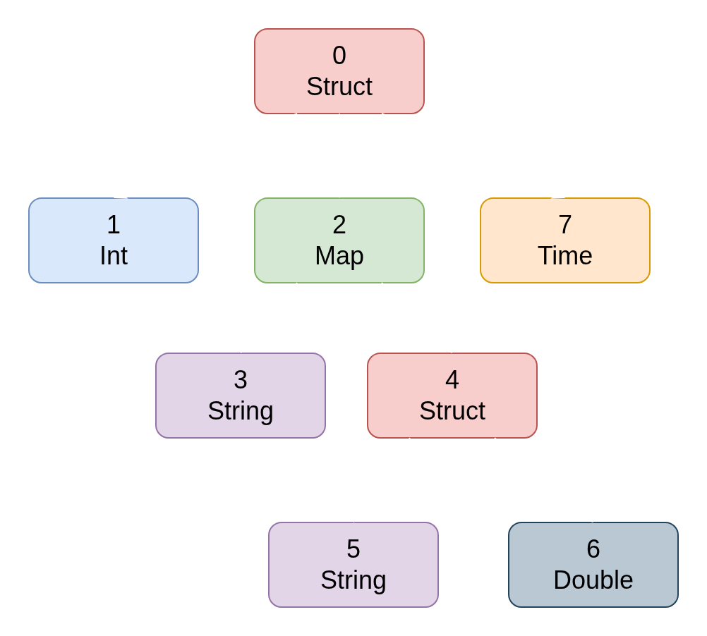
The columns in the file would form the following tree:
Why ORC?
- Really efficient compression - It saves a lot of storage space
- Support for ACID transactions - ACID Support
- Predicate Pushdown efficiency - Pushes filters into reads so that minimal number of columns and rows are read
- Schema evolution and merging
- Efficient and fast reads - Thanks to built-in indexes and column aggregates, we can skip entire stripes and focus on the data we need
Final Words
Understanding how big data file formats work helps us make the right decision that will impact efficiency and scalability of our data applications. Each file format has its own unique internal structure and could be the right choice for our storage strategy, depending on the use case.
In this article I've tried to give a brief overview of some of the key points that will help you understand the underlying structure and benefits of popular big data file formats. Of course, there are many details which I didn't cover and I encourage you to go through all of the referenced material to learn more.
I hope you enjoyed reading this article and, as always, feel free to reach out to me if you have any questions or suggestions.
Bonus
AliORC (Alibaba ORC) is a deeply optimized file format based on the open-source Apache ORC. It is fully compatible with open-source ORC, extended with additional features, and optimized for Async Prefetch, I/O mode management, and adaptive dictionary encoding. Ref: AliORC: A Combination of MaxCompute and Apache ORC.
Resources
- Big Data File Formats
- Performance comparison of different file formats and storage engines in the Hadoop ecosystem
- Databricks - Parquet
- All You Need To Know About Parquet File Structure In Depth
- Apache Hive - ORC
Footnotes
-
Volume, Variety, Velocity, and Veracity ↩
-
The father of Hadoop and Lucene. Ref: Wikipedia - Doug Cutting ↩
-
A month later, the Apache Parquet format was announced. Ref: Wikipedia - Apache ORC. ↩